|
|
| 
|
Nyquist
Frequency
The Nyquist frequency, named
after electronic engineer Harry Nyquist, is half of the sampling rate of a
discrete signal processing system. It is sometimes known as the folding
frequency of a sampling system. An example of folding is depicted in Figure
1, where fs is the sampling rate and 0.5 fs is the corresponding Nyquist
frequency. The black dot plotted at 0.6 fs represents the amplitude and
frequency of a sinusoidal function whose frequency is 60% of the sample-rate
(fs). The other three dots indicate the frequencies and amplitudes of three
other sinusoids that would produce the same set of samples as the actual
sinusoid that was sampled. The symmetry about 0.5 fs is referred to as
folding.
The Nyquist frequency should
not be confused with the Nyquist rate, which is the minimum sampling rate
that satisfies the Nyquist sampling criterion for a given signal or family
of signals. The Nyquist rate is twice the maximum component frequency of the
function being sampled. For example, the Nyquist rate for the sinusoid at
0.6 fs is 1.2 fs, which means that at the fs rate, it is being undersampled.
Thus, Nyquist rate is a property of a continuous-time signal, whereas
Nyquist frequency is a property of a discrete-time system.
When the function domain is
time, sample rates are usually expressed in samples/second, and the unit of
Nyquist frequency is cycles/second (hertz). When the function domain is
distance, as in an image sampling system, the sample rate might be dots per
inch and the corresponding Nyquist frequency would be in cycles/inch.
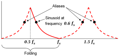
The black dots are aliases of each other. The solid red line is an
example of adjusting amplitude vs frequency. The dashed red lines are
the corresponding paths of the aliases.
|
| |
|
